| Conditional code, and condition Flags: Link |
| Functions, Interrupts (Stack memory): Link |
| Loops, and repeat Link |
| Array's, and data structure: Link |
| Complications, and Conclusion: Link |
Pre compiled binary.
A Pre-compiled binary runs on an ecosystem of processors that are the same architecture type.
This is how Windows, DOS, Unix, Linux, and macOS work.
The loader for the application is designed to dump the pre-compiled binary into RAM.
The CPU is meant to run the program instructions as is without recompiling the code.
The systems have been initially designed to target x86 cores.
Which mainly meant AMD, Intel cores, and some off-brand x86 cores that run x86 instructions.
You can learn some of the basics of machine code and processor architecture the following link.
Dynamically generated code.
Such as Java, Scripting languages, emulators (JIT/Interpreter).
These forums of code store instructions stored in the file that are not understood by the CPU directly.
In java it is called java byte codes. As loading, a new part in an APP, or game takes more time than a pre-compiled code.
In the case of an emulator, it only changes the instruction encoding if it does not match the CPU architecture type in your system, or we can interpret each instruction using arithmetic in code which is very slow.
The advantage of this is that you can change the byte code commands into different processor instructions.
The main binary that does all the work is called a JIT compiler or interpreter.
The JIT compiler or interpreter is built-in pre-compiled binary code to run fast on the target architecture type.
However, if you use the JIT compiler or interpreter as the base of your operating system for loading applications, that is dumb and a bit slower on performance.
Cases in which dynamically generated code speeds stuff up are.
Dynamically generated AI (Artificial intelligence) code. This is somewhat different as it takes information in to generate changes to itself.
There is also self-modifying code that can make modifications to itself to save time in algorithms and loops.
Data types.
The basic arithmetic types such as Integers numbers, floating-point, text data, do not change between CPU architecture types.
The data types for data processing and doing math arithmetic and text are standardized.
Also, everything is in bytes. Thus numbers are in different word sizes using bytes.
You can learn about them following: link.
The most java has to do is compile the program’s instructions into instructions the target CPU architecture uses.
The processor should be able to process the standard primitive data types.
Translating to code.
The steps you put into code are similar septs in machine code. It just is a little harder to follow.
What will change is you will see it moves a number into a register and adds it with the value, writes it back to memory at the location of your variable.
The first thing that will be noticeably missing is the names of your data types.
So when you see add, subtracts, and other operations that you would typically do in code.
You give them temporary variable names. Until you know what they were intended for in the steps of the code.
You also have to pick a language syntax that you are comfortable with. Such as JavaScript, or C.
As you define what the steps are doing, it does not matter which language you target to write the steps back out in.
You also should be able to distinguish some of the basic built-in methods in a programming language.
If you see a number being divided by ten till no remainder. Then you know it is the toString method. Which converts the number to a base-ten number.
Uses graphics to draw the character values using the standard text format. However, you could write out the complete logic of the code.
It will still compile back out fine. However, it makes it easier to read if you recognize the built-in methods.
Arithmetic comparison.
Normally in programming languages. You can compare things in a single line of code. However, comparison is done using arithmetic logic.
All CPUs have to do it in a few steps regardless of the CPU type.
A processor’s arithmetic unit has outputs zero, sing, carry, overflow. So do calculators.
These outputs are saved into a flag register from the arithmetic circuit per every arithmetic instruction.
A simple ALU design is that of the 74181 which started the design of single chip CPU’s. Following: link.
All processors today have very small ALU’s which are designed to do all arithmetic operations. The small size is achieved by having the S inputs change the logical combination between the input to output.
Thus, you need to know the correct values to set the S inputs to generate the right logical combination between the input to output to do an ADD or subtract.
The pin that is “A = B” is the zero flag from the 74181, and P is parity, meaning output is odd or even.
We also have carry as a pin output. The sing is just a straight connection from the last binary digit output. Modern ALU’s are 8 in size today. Thus are grouped together in word sizes.
A CPU like an x86 one will have a comparison instruction. The compare instruction does a subtract between two numbers without writing the result.
We could use subtract instead on any CPU, but using compare is better if you do not wish for the value to be subtracted and only want to compare.
Now the zero output is set when the output is all 0 from any arithmetic operation. Which is just a inverter with an and gate at the output.
This means both values are the same such as 7489328 - 7489328 = 0, which sets zero to active in the flag register.
If the subtracted value is smaller, then the last binary digit would be borrowed, causing the last binary digit to be set.
This sets “sing = 1” as in negative value. If the value was grater than “sing = 0”.
Comparing the flags after subtracting or compare allows us to create less than, greater than, equal to, or less than equal to, and greater than equals to.
This is the standard way comparison is done arithmetically by all CPUs.
The programmer is not used to comparing something first and then doing a conditional jump.
A processor jump in an x86 core will only jump to the location if the flags are set to the correct value after comparing, subtracting, or any arithmetic instruction.
Otherwise, the instructions after the jump will run.
On an ARM core, all instructions have a condition code. This means the instruction might not run relative to the arithmetic results of the past instruction.
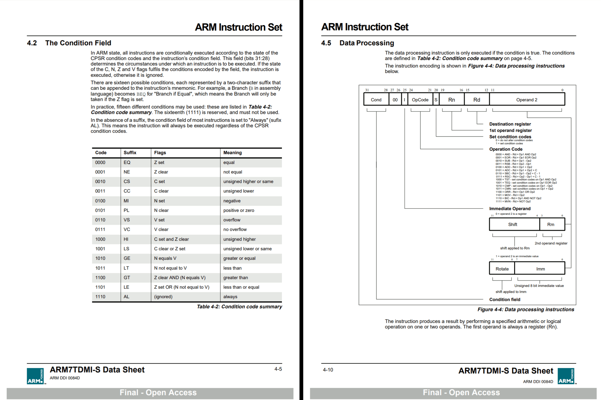
We can also force the Arithmetic output flags not to be saved using the S-bit. This allows us to make some very interesting code on an ARM core.
This allows us to build the logic for various arithmetic operations in code using conditions parried with arithmetic.
This allows ARM cores to have few operation codes but do just as much as x86 cores.
This has allowed ARM to use fewer transistors and runs on low-power devices.
On an x86 core, we have dedicated instructions for everything Arithmetic-based.
An ARM may spend a few more instruction cycles doing an operation an x86 can do in one instruction cycle.
The only conditional instructions on an x86 core are the jump instructions. Generally, a compiler will write out the steps in your code in each separate if statement.
It then links them together linearly. So it is vital to map the conditional jump locations as these will tell us where code separates into IF statements.
While on an ARM core. It can be instructions with conditions to make a combinational arithmetic operation or program logic.
What we call a jump instruction on an x86 core is called branching on an ARM. An ARM conditional branch works the same as an x86 conditional jump.
So mapping ARM conditional branches reviles the programs if statements and separations.
Control unit.
The Arithmetic unit does most of the operations. However, the control unit is the most important.
The control unit is what does the Compare instruction. The control unit does the subtract with ALU but sets the write to register off.
This allows us to compare without writing the subtracted result. In earlier x86 cores, the control unit orchestrated a multiply or divide as multiple ALU instructions as well.
Modern ALU’s have seven adders in front that allow 8 bit multiply or divide in one clock cycle. The adders can be switched off or on.
This allows x86 cores to do fast multiply or divide. Also made 32/64 bit multiply or divide much faster.
As we can make the circuit smaller, we can include a full 32/64 div/mul in one clock cycle.
Because of the control unit, we can also choose the carry flag to be given into the carry input. This creates instruction add and carry, and subtract and barrow (carry flag), which allows us to add or subtract numbers as large as we want.
Without the control unit, we would also not have conditional instructions, which makes the CPU programmable.
Also, it is important to know that the combinational ALU opcodes can be different than the codes the control unit uses.
Lastly, it is essential to make sure your CPU is compatible with software written in x86 core code instructions, or ARM depending on the type you build.
Also, floating-point instructions are built off of the ALU. Float numbers are added regularly; however, they are shifted relative to the exponent.
So floating point operations using IEEE floating point are easy to implement; however, they are a bit slower even on modern CPU.
What has changed the most on CPUs is how small we can make transistors, and how close together the connection are is what makes CPUs so fast today.
Method calls, and function calls.
x86 cores have a unique way of calling a method or function in code.
The CALL instruction writes the current position the CPU is at in the code into RAM then jumps to location.
So the CALL operation is two operations in one. The RET operation reads the number wrote into RAM and then jumps back to that location.
The instructions that came after the CALL operation continues.
RET is short for return back, which RET is a read and jump.
CALL/RET uses a register called the stack pointer as the location to write and read the value.
If you change the value of the stack pointer register, then use RET. We may not return back to the correct location.
Suppose you do change the value of the stack pointer register to do an add or some arithmetic operation before using RET. Make sure you set it back to what it was.
Another thing you have to worry about is instructions PUSH and POP. Suppose you use instructions PUSH or POP before RET. You also may not end up back.
The instruction PUSH writes the value of a register to the location of the stack pointer.
The operation POP puts a value from the stack pointer location into a register.
AS you write bytes at the location of the stack pointer register using PUSH, the stack pointer is subtracted by the bytes you write.
AS you read bytes at the location of the stack pointer register using POP, the stack pointer is added by the bytes you read.
Everything you PUSH must POP in order. This way, RET will return back to the correct location.
There are some tricks to this, though. Say you build a method that takes two integers as input.
You may see these two integers get PUSHED onto the stack pointer location before CALL.
During the method, you may see it use the stack pointer plus 8 as integer one input, plus 12 as integer two input while the other 8 bytes is the RET location.
You will see this lots in x86 binaries.
Also, print stack trace prints the stack of the methods that are last called by locations in the stack register location. Some programming languages support this feature.
It is also essential that the stack pointer register is set far enough away from the program instructions so that it does not write over program instructions.
So when you create functions/methods in code. They get compiled out the same way.
Some programming tools let you inline the code. This means the compiler puts the code for your method in with the rest of the code instead of doing a CALL.
This is done to make the code faster. This can triple to double the size of the binary program depending on how many places you use the function/method in the program.
Interrupts vs CALL.
Short for INT followed by an interrupt number. These are also the same as a CALL instruction.
One of the Traditional things an operating system does is set up a list of locations at address 0 and up.
The first number is INT 00, and the second is INT 01, and so on.
The instruction INT 03 will read the fourth number. The number is the JUMP location.
Before the CPU goes to the location, it writes the location it currently is at in memory.
It stores the location the interrupt happened at the location of the stack pointer register, the same as the CALL instruction.
At the end of the code, an RET is used. This allows your code to resume after the interrupt.
Interrupts are just a fancy CALL instruction that uses an array of locations at address 0 in RAM.
Interrupts are not used much anymore by modern operating systems. Windows 10 still loads some methods into the interrupt list.
However, they are rarely ever used. The regular CALL instruction is preferred over Interrupt CALL.
You can still look at the map of INT codes: DOS API INT Setup vector.
Windows Vista and earlier still supported the entire DOS API. Windows 10 still has a few Interrupts that load in, but very few.
I used to write binaries in pure binary code with a hex editor. Such as print a small message using “int 21”.
I also did simple graphics in video memory for fun only when I got really bored. This was also good practice.
Bellow, I will show a sample COM file.
B4 09 BA 08 01 CD 21 C3 48 65 6C 6C 6F 20 57 6F 72 6C 64 24
You can start applying your skills here to read it. You already know basic x86 instructions B0 to B7 are 8 bit MOV operations. Thus instructions B8 to BF are 16 bit MOV.
Just looking at this COM code. You can see MOV operation “B4” using register 4, setting the register AH to 09.
You then can see “BA” which is the 16-bit register DX. The two bytes 08 01 are read in little-endian byte order as value 01 08.
We then see instruction “CD” which is the interrupt instruction code. We then see the number 21 after it, which is interrupt 21.
Lastly, “C3” is the return code. This returns back to the operating system after the code is run.
Thus if AH is 09, and we use interrupt 21. Then the value in DX is used as the address to our text-based message.
All COM files start at 0x100, so the value in DX is 0x108. So if you count 8 bytes from the start of the code, you will find the position to the message.
Which is 48 65 6C 6C 6F 20 57 6F 72 6C 64 24. In UTF8 text standard, this is “Hello World$”. The dollar sign marks the end of the text for int 21 with AH 09.
A COM file had no header or setup information. A COM is directly run as CPU instructions in 16-bit mode. After windows vista, MS removed all the necessary interrupt functions. This made the COM files unrunnable.
To run a COM file after windows vista. You need to used dos box. Which dos box simulates the “int” function calls.
It is still good practice in learning to write pure binary applications in x86 core code without any coding tools.
Loop, and repeat.
x86 cores also have loops and repeat instructions. These small things can be very useful.
The loop instructions are the same as your jump instructions. Except it jumps and subtracts the counting register by one.
The LOOP instructions should always locate back to a previous instruction location or set of instructions before the LOOP/JUMP instruction is reached again.
Once the counting register is 0, then the LOOP instruction no longer jumps back, allowing the next instructions to run.
The counting register should be set to the number of times you want to loop.
The Repeat prefix can be used before any x86 data processing operation. The REP prefix will repeat the next instruction until the counting register is zero as well.
The repeat prefix is much more efficient than a loop if only you want to do the same instruction multiple times.
There are a few special move operations for moving data around. They are operation codes A4, A5. These instructions automatically use two RAM address locations using two registers.
A4 = MOVS BYTE PTR [RDI],BYTE PTR [RSI]
This instruction does not let you encode which registers to use.
When you are using instruction MOVS, SI is considered as the source register, while DI is considered as the destination register.
The instruction MOVS adds one to both SI and DI as it writes one byte from SI location to the location of DI.
If we run this operation a bunch of times. It can move data from one spot of memory to another.
So by using the repeat prefix to repeat the next instruction. We can have this move data as large as we want to the value we set in the counting register.
The repeat prefix is byte code F3 hex. So you may see the byte sequence F3 A4. You can also come up with ways in which the repeat prefix may be useful with one instruction.
F3 A4 = REP MOVS BYTE PTR [RDI],BYTE PTR [RSI]
In ARM, we have a special instruction called a block copy instruction to achieve this same operation.
Array, and data structures.
There is a limited number of ways of building an array in machine code. Generally, the best way to create an array is to think of the word size of the numbers we wish to store in the array.
In the case of an array made using bytes. Each next byte is a new index in the array. The start position of the array in memory is called the base.
The selected byte is then base plus index. When index is 13, then the 13th byte is read. This allows us to read which element we want from the array directly or write the new value.
A simple array is like this.
MOV RBX,0000000403700080
MOV RDI,0000000000000007
ADD BYTE PTR[RBX + RDI],78
We add 78 to the array index 7. So RBX is the base of the array 403700080. We add 7 to 403700080 for the 7th byte across as the address.
If we make this into a loop and add the RDI register by one each time. We are effectively adding 78 to all indexes after index 7.
Let’s say we have an array where each number in the array is 8 bytes big.
MOV RBX,0000000403700080
MOV RSI,0000000000000009
MOV RDX,QWORD PTR[RBX + RSI * 8]
In the above example, we read the 9th 64-bit number into the RDX register. We then can start comparing the 9th number or make it a loop.
Since each index can be two bytes instead of one, the x86 core also lets you multiply the index register by 2, 4, or 8.
We can pick any two registers to add together as an address location. Thus the base register is more or less just a historical name.
Now you may be wondering how we create arrays with multiple dimensions in linear space.
MOV RBX,0000000403700080
MOV RSI,0000000000000009
MOV RBX,QWORD PTR[RBX + RSI * 8]
MOV RSI,0000000000000002
MOV RDX,QWORD PTR[RBX + RSI * 8]
This time the first array stores the location to another array. So we are asking for the location to the 9th array.
We then set RBX to the location of the 9th array. We then set RSI to 2, which moves the value into the RDX register.
This is how two-dimensional arrays are done in memory. In code it would look like this MyVal = MyArray[9][2].
In the case of a three-dimensional array in linear space.
MOV RBX,0000000403700080
MOV RSI,0000000000000003
MOV RBX,QWORD PTR[RBX + RSI * 8]
MOV RSI,0000000000000007
MOV RBX,QWORD PTR[RBX + RSI * 8]
MOV RSI,0000000000000002
MOV RDX,QWORD PTR[RBX + RSI * 8]
In code it would look like this MyVal = MyArray[3][7][2]. We let RBX locate to each next array.
When we write a 3D or 4D array in machine code, we have to be very careful with the locations of each array.
Because we have to write out each location, RBX will be set. Thus it must line up to the base position of each array.
In a programing language, the coding tool will line up the linear space for your array. Also, the more dimensions you add to your array the slower your code may become.
We can also write the array out as follows.
Location = MyArray[3]
Location = Location[7]
MyVal = Location[2]
Thus programming languages let us store the pointer locations to an array. This improves performance if we wish to iterate over one array location.
Data structures.
Now let’s say we wish for each array element to hold more than one value. This is called a data structure.
Now lets say we create a house data structure. We want to store a byte that is 0 to 255 for which type of flooring.
We want a byte for which kind of wallpaper that is 0 to 255. We want another byte that is 0 to 255 for the type of lighting.
In programming languages, we can specify things like this.
House
{
  byte flooring = 0;
  byte walls = 0;
  byte lighting = 0;
};
We can specify our array as follows House[][][] myArray = new House[10][10][10];.
When we address each thing in the data structure, it goes as follows.
MOV RBX,0000000403700080
MOV RSI,0000000000000003
MOV RBX,QWORD PTR[RBX + RSI * 8]
MOV RSI,0000000000000007
MOV RBX,QWORD PTR[RBX + RSI * 8]
MOV RSI,0000000000000002
MOV RBX,QWORD PTR[RBX + RSI * 8]
MOV R8,QWORD PTR[RBX]
MOV R9,QWORD PTR[RBX + 1]
MOV R10,QWORD PTR[RBX + 2]
This time the third dimension points to our data structure location, which consists of three-byte values that go in order the way they are defined.
The x86 address system lets us add an offset to our address location called a displacement. The register R8 is flooring. The register R9 is walls. The register R10 is lighting.
In a programming language, it looks like this.
MyHouse = MyArray[3][7][2];
MyVal_1 = MyHouse.flooring;
MyVal_2 = MyHouse.walls;
MyVal_3 = MyHouse.lighting;
Thus we can iterate over the 3D array of 3D placed houses.
However, the best way of writing this code is to make a one-dimensional Array with each house containing an x, y, z position that it is placed.
We also generally do not want to make a custom data structure if we do not need one.
This completes the complete introduction to the x86 Scale index base system.
Data structures can also exist as a single location as well in a program or as the header data structure at the start of a binary file.
In which the data structure defines the attributes associated with the file type. Or if you only want to use the data structure as a single variable in your code.
Programming tools and programming languages allow us to give things names rather than being locations once compiled out.
All the different ways of iterating and pointing to data are usable from coding tools without manually organizing the arrays and variables in your program or code.
Lastly, your standard primitive data types are your building blocks for custom data structures and arrays. The primitive data types can be processed using the basic CPU arithmetic/FPU instructions.
Adding methods to data structures.
Programming languages can let you define methods inside of a data structure, which are called Objects rather than data structures.
This allows you to do thing like this MyHouse.wallAndFloorSame().
This can be a simple method that reads what flooring is and then sets the walls to the same byte value. Or you could do MyHouse.wallsRandom().
This is done to organize your code better. A compiler may not write out the instruction as a call. So what ends up happening is the location is written to.
MyHouse.wallAndFloorSame() can end up changing back into Location.Thing0 = Location.Thing1.
Some compilers will only write it out as a standalone method if used in more than one location of your code and is a large set of steps.
In the reverse process, we can lose which methods belong to an object and lose the names things are given as they are locations only.
The code we end up with compiles back out and runs the same, just that it might not match exactly how you wrote it.
x86 register naming scheme.
Originally all x86 general arithmetic registers had no names.
Register 4 was used with arithmetic operations just like the other registers. However, register 4 also was used with instructions PUSH/POP/CALL/RET.
In which register 4 became known as the stack pointer register (SP for short). In which SP is still a general arithmetic register.
Just that is is called stack pointer, because it is used as a location, for operations PUSH/POP/CALL/RET.
The same applies to the counting register, destination, and source.
All registers in ARM go by number code. As there are no special case instructions that use a particular register by default.
In x86, Register 3 is used by default to store or send a value between a port number using input or output instruction codes 6C, 6D, 6E, 6F.
So register 3 became known as the data register.
Complications/Conclusion.
The only thing that can become complicated is arithmetic paired with conditional jumps. Rather than compare and jump (Or ARM branch).
This can make it tricky to reconstruct the original if statements in code.
The easy part is defining function calls and variables. Giving the variables/locations a meaningful name for what they are used for can be tricky sometimes.
So generally, we can get close to reconstructing the source code of a C program, or C++, or can change it to any other language syntax.
When it comes to code wrote only in machine code. We can convert said instructions and word sizes of add and subtracts to variables, data structures, and to actual steps in code.
Meaning there is not much difference between machine code and coding in a programming language.
You can choose to write out your data types one at a time before your code or have the compiler write out the data types as a list at the start of your code. Each spot a variable is used will be referenced from there.
A programming language is a syntax for organizing your code better. All the ways of dividing up memory, iterating data, or looping through things have to be structured; otherwise, the machine code must change during a loop.
The programming language allows you to name things and add comments in the code explaining a section, which does not exist in the binary. Variable names and data structure names no longer exist.
A programming language also uses {, to } brackets to specify the start and end of a set of instructions. Which are compiled out as separate codes that can be jumped to. They are linked together by if statements, and loops.
Loops are straightforward to identify. It can be a jump that jumps back till some condition, or the LOOP instruction till counting register is 0.
Data structures are easy to identify, and so are arrays.
Also, ARM has an addressing scheme that is used with its built-in barrel shift on every instruction. Just it is not as good as the x86 index and base address system.
A programing language is more or less just a style of syntax you like. Thus it also depends on if you like a big programming language with lots of source code files that do everything for you, or if you like writing out everything yourself.
Also you may enjoy the following on Obfuscated code: Link. Although you will encounter very few binaries that use the tricks discussed in this document today.
The tricks done to make a machine code harder to read are usually only done by viruses. So generally, it is straightforward to read machine code programs back into data types and method calls.
Security issues.
Giving away your binary applications using licensing controls in the code is more or less a waste. Such as software trial licensing.
It is not any harder to rewrite and take a program apart as it is having the source code of the program. It is the equivalent of giving away your program for free.
It is also not hard to set the score to what you want in a game. There is nothing magical about said tasks. It also is easy to follow the starting of an operating system.
There is not much difference between machine code and programming language. Also, machine code is the same between systems.
A programming language is only an syntax to organize your data types by name instead of the location in the binary.
Even the entire windows operating system is built-in C/C++ as well now.
Writing better and faster code starts with how you simplify and organize the methods and how efficient your data types and steps of your code are.
There also is no such thing as a secrete algorithm or format as you can easily find any algorithm in any compiled binary.